How to Create a Pivot Table in Excel

Pivot tables are an incredibly useful tool for organizing, summarizing, and analyzing large amounts of data in Microsoft Excel. 

With a pivot table, you can quickly and easily transform complex datasets into meaningful insights that can inform business decisions. 

So let's walk through a step-by-step guide on how to create a pivot table in Excel.

Step 1: Prepare your data

The first step in creating a pivot table is to ensure that your data is properly formatted.

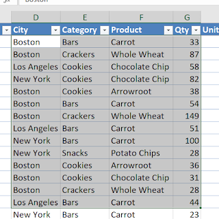
Your data should be in a tabular format, with columns that have clear headers and consistent data types. Additionally, your data should not contain any empty rows or columns.

Step 2: Select your data

Once your data is properly formatted, the next step is to select the range of cells that you want to include in your pivot table. 

You can do this by clicking on the first cell in your data range and dragging your mouse to the last cell.

Step 3: Create a pivot table

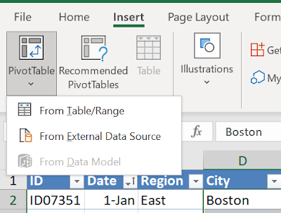
To create a pivot table, go to the Insert tab in Excel and click on the PivotTable button.

This will bring up the Create PivotTable dialog box.

Step 4: Choose your data source

In the Create PivotTable dialog box, you will need to select your data source.

This can either be the range of cells you selected in step 2, or an external data source such as a database or another Excel workbook.

Step 5: Choose where to place your pivot table

After selecting your data source, you will need to choose where to place your pivot table. 

You can either place it in a new worksheet or in an existing worksheet. 

If you choose to place it in an existing worksheet, you will need to select the cell where you want your pivot table to start.

Step 6: Design your pivot table

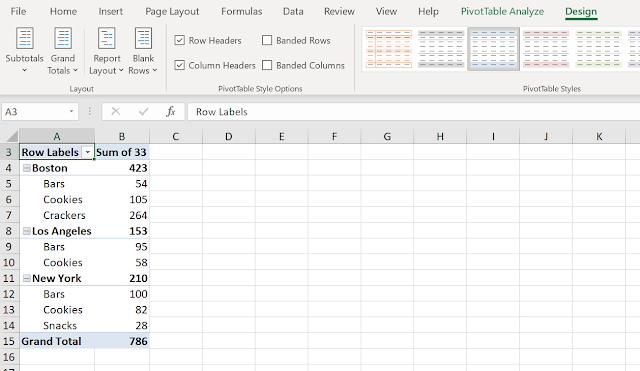
Once you have created your pivot table, you can begin designing it to meet your needs.

To do this, you will need to drag and drop the fields you want to include in your pivot table to the appropriate areas. 

The areas in a pivot table include:

• Rows: This area contains the fields that will be used to group your data vertically.
• Columns: This area contains the fields that will be used to group your data horizontally.
• Values: This area contains the fields that will be used to summarize your data.
• Filters: This area contains the fields that will be used to filter your data.

To add a field to your pivot table, simply drag it from the field list on the right-hand side of the screen to the appropriate area in the pivot table.

Step 7: Format your pivot table

After designing your pivot table, you can format it to make it more visually appealing and easier to read. 

To format your pivot table, you can use the options in the PivotTable Styles gallery on the Design tab. 

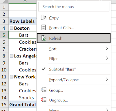
You can also customize the layout and formatting of your pivot table by right-clicking on any cell in the pivot table and selecting the appropriate options from the context menu.

Step 8: Analyze your data

Once your pivot table is designed and formatted, you can begin analyzing your data. 

You can do this by using the various features and tools available in Excel, such as filters, slicers, and calculated fields. 

• Filters allow you to limit the data displayed in your pivot table based on specific criteria. 
• Slicers provide an interactive way to filter your data by displaying a set of buttons or a scroll bar that you can use to select specific items. 
• Calculated fields allow you to create new fields in your pivot table by performing calculations on existing fields.

Step 9: Refresh your pivot table

Finally, it's important to note that pivot tables are dynamic and can be updated as your data changes.

To refresh your pivot table, simply right-click on any cell in the pivot table and select "Refresh" from the context menu. 

This will update your pivot table with any changes made to the underlying data.

( Data samples : https://www.contextures.com/xlsampledata01.html )